Quick Navigation

<= <= Return to the µOpenSPIM starting page
<= Return to Image acquisition

Acquisition Controls

The following image will introduce you to the location of all available controls to set up an imaging session.

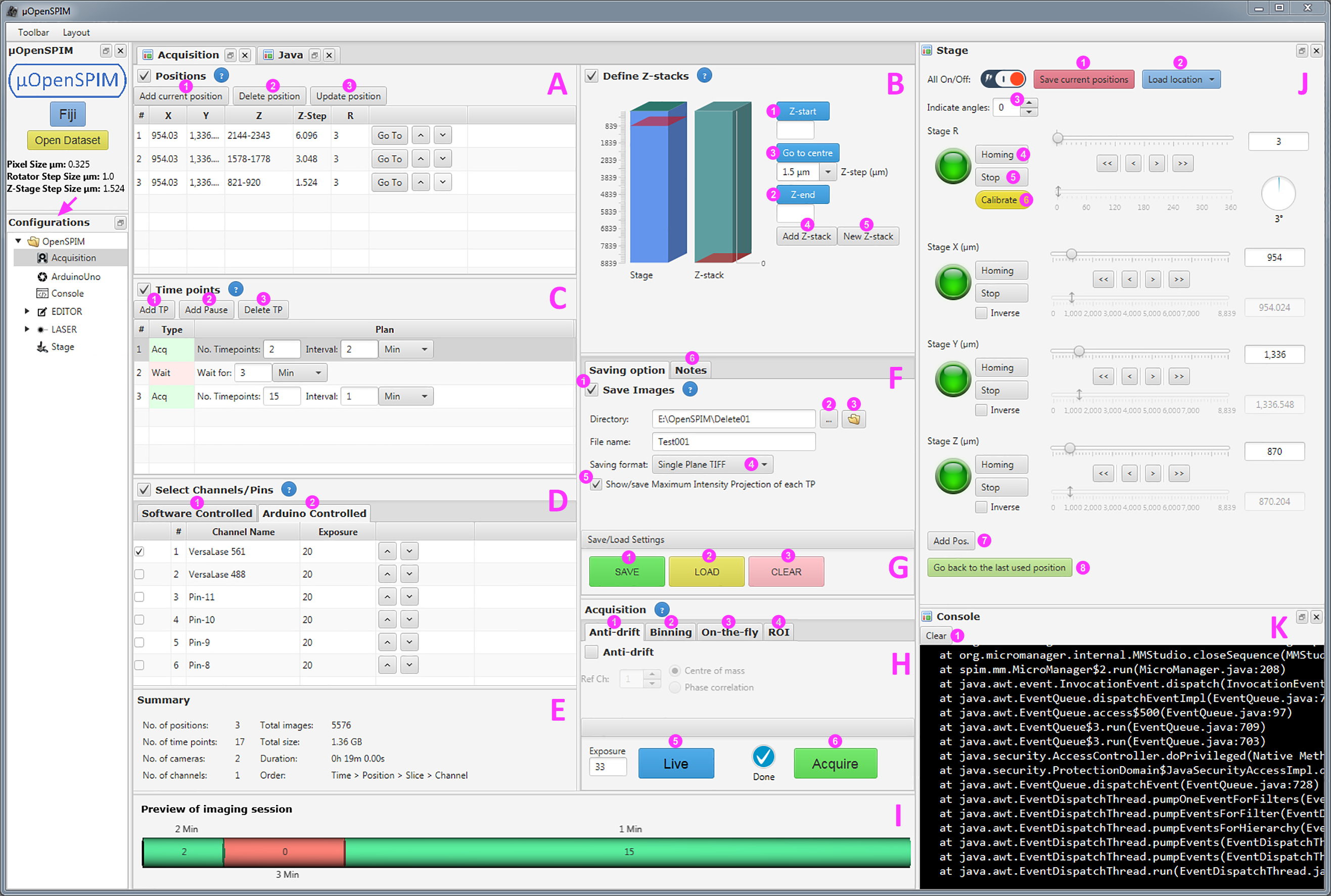
(A) Positions
This table shows the list of predefined positions, which will be acquired at each time point. There might be multiple positions or just one. A position is defined by the location where the four motorized stepper motors (X, Y, Z, and R) will move before acquiring an image or stack at a given time point.
In case of an 3-dimensional stack, the Z stage will have three location values: Z start and Z end location values, both defining the total volume of the stack, and the Z step size value, which specifies the total amount of slices within this volume, whereby each slice is one image.

1. Add position: Clicking this button will add a row to the end of the table with the current X, Y, Z and R coordinates.
2. Delete position: Clicking this will remove a highlighted row from the table. You can click and drag rows and move them up and down by using the arrows at the end of the row.
3. Update position: Clicking this button will update the selected position according to the current 4D-stage positions (X, Y, Z, R).

(B) Define Z-stacks
Here the beginning and the end of a new stack together with its Z step size can be specified using the Z stage. One has to first find the sample and a centre it in the field of view. By navigating through the sample along the z-axis the beginning and end of a z-stack is specified.

1. Z-start: Clicking this button will mark the current z stepper motor position as the beginning of a desired z-stack.
2. Z-end: Clicking this button will mark the current z stepper motor position as the end of a desired z-stack.
3. Go to centre: Clicking this button will move the stage Z into the centre of the defined z-stack.
4. Add Z-stack: Clicking this button will add a row to the end of the positions table that will include the X, Y, and R positions together with the two z-stack positions (Z-start and Z-end) and the Z step size value.
   

• It is possible to manually change any positional values by double-clicking on one of the positional entries. Note that this can be done during an ongoing imaging session.

5. New Z-stack: Clicking this button will clear all previously locked Z-stack values in order to define a new Z-stack.
   

• It is possible to manually change any positional values by double-clicking on one of the positional entries. Note that this can be done during an ongoing imaging session.

In order to overwrite all positional values with the current positions of the stepper motors simply select any previously created position entry and press the “Update position” button.

(C) Time points
This table includes the information how often the predefined positions should be acquired. A time point can be specified once or many times for long term time lapse recordings. In case 3-d stacks are acquired across a given period of time, the imaging process is referred to as 4d-Microscopy.

1. Add TP: Clicking this button will add a row to the end of the time points table where the number of time points and their recurrent intervals can be specified.
2. Add Pause: Clicking this button will add an acquisition break to the end of the time points table.
3. Delete TP: Clicking this will remove any highlighted row from the time points table.

(D) Channels
A typical channel is a laser of a given wavelength illuminating the sample during acquisition. In case an Arduino UNO is in control of one or several lasers, they all must be wired to one of the digital output pins. It is possible that a channel represents a different device other than a laser. Alternatively, lasers can also be controlled by the Software, which in our case is µManager. Do find out more about Software versus Hardware controlled imaging, click here.

1. Software controlled Click Add channel to add a new channel to the table. Several channels can be added to the table.

• Click into the drop-down menus to change Camera and the correct Shutter for the intended laser line.
• Double click on the exposure value of any added channel to change it.

2. Arduino Controlled: Simply select one or several of the available channels (Pin8 to Pin13) that are under the control of the Arduino-Shutter. Channel Names can be changed in the Arduino UNO configuration table.
   • Double click on the exposure value of any added channel to change it.

(E) Summary
This table provides a summary of the final imaging session with its current settings.

(F) Saving options

1. Save images: If ticked acquired images will be saved to the hard disk.
2.   Clicking this button will allow you to specify an Output directory.
3.   Clicking this button will open the specified Output folder.
4. Saving format: 
   • Choose Single Plane TIFF to save every image individually.
   • Select OMETIFF Image stack to save every time-point as an individual stack including all channels as an ometiff file.
   • Select N5 format to save your acquired data in the N5 format, which allows images to be available in multiple resolutions and can be written in parallel. More info on N5 can be found here.
5. Show/save Maximum intensity Projections of each TP: We advise to tick this option for long time-lapse recordings. It can be very useful to have a first impression of how well an imaging session goes or went, particularly if large SPIM data is acquired where generating MIPs after imaging is completed can be very time-consuming.
6. Here notes can be written down, which will be saved as an additional Note.txt file into the Output directory.

(G) Save/Load settings
All input settings created by the user including Positions, Time points and Channels can be saved here and loaded again at a later time point.

1. Click SAVE to save all acquisition settings as an .xml file.
2. Click LOAD to load previously saved acquisition settings.
3. Click CLEAR to clear the Acquisition panel from all settings and tables.

(H) Acquisition
After all positions and number of time points have been specified, it's almost time to start imaging. However, there are still a few options worth considering before starting the acquisition process such as ROI, Anti-Drift and Binning. It's also worth checking one more time if the correct saving format has been chosen and whether Maximum Intensity Projections should be generated on the fly.

1. Anti-Drift: Click the Anti-drift tab to enable it with the aim to prevent the sample from leaving its initial predefined position. One can choose between Phase Correlation (whereby entire volume of a 3d-stack is taken into account) or Centre of Mass (whereby drifts are only corrected in x, y but not in z). Note that high concentrations of fluorescent beads surrounding the sample may disarrange the Anti-Drift functionality.
2. Binning: Different binning options can be selected before acquisition, e.g. 2x2 or 3x3 binning. Higher Binning settings combines the charge of more pixels, which increases the signal to noise ratio (SNR) and results in higher camera frame rates but on the expanse of pixel resolution.
3. On-the-fly: On-the-fly will enable the “process()” method of a running script, which can be created or edited within the Java Editor (Editor > Java).
4. ROI: Within this tab a region of interest (ROI) can be specified and applied to the field of view of the camera. The region is specified in the preview window of µManager. Select the Rectangle tool and create a selection inside the preview window. The window will open up by clicking Live view. When the ROI is specified, click the Apply button.Live: Clicking this button will toggle the camera into live view. The exposure values can be changed below.
5. Acquire: Clicking this button will start the currently set up imaging session.

(I) Preview of imaging session
Here a simple schematic overview is given showing the current list of time points that have been set up.

(J) Stage
Here you can move the four stepper motors of the 4D-stage Stages (X, Y, Z, R), calibrate the rotational stepper size (R Stage), save and load current positions and inverse the axis of the x and y stage, which might be crucial for the Anti-Drift to work correctly.

1. Save current position: Click this button to save the current position of the stage. It will be added to a list.
2. Load location: Click this button to Load a previously saved stage position from a list.
3. Indicate angles: Indicate here the number of angles you wish to acquire during a single time-point. The angles will then be indicated above the rotational stage (Stage R).
4. Click Homing on one of the four Stages to move the stepper motor back to its home position.
5. Click Stop to immediately stop a stepper motor.
6. Calibrate: Click this button to calibrate the R Stage in case the 360 degrees do not correspond to a full revolution of the sample holder.
7. Add Pos. Clicking this button will add a row to the end of the Position table using the current X, Y, Z and R coordinates.
8. Go back to the last used position Clicking this button will move the stage to the previous position.

(K) Console
The console window can be useful to see what is going on in the background of the plugin and to spot error messages.

1. Clicking Clear  will delete all written content.