Fusion
Registered multi-view OpenSPIM data need to be fused into a single output image in order to achieve complete coverage of a large specimen. Fusion means here combining information from different views in areas where the views overlap. Several strategies to do so exist, many are published (TBD). We will focus here on the two fusion methods implemented in Fiji - the content based multiview fusion and multiview deconvolution.
Note that fused data are different, not necessarily better compared to raw SPIM data. Both fusion algorithms described here potentially deteriorate the quality of the data in some respects while improving other aspects. We will discuss the fusion artifacts in the respective sections. However it should be said that sometimes it is beneficial to NOT fuse the data at all and perform analysis on the raw registered image stacks (for example segmentation of cells in the individual views and reconciliation of the results in the segmentation domain). In this tutorial on browsing we will describe how to view raw registered multi-view OpenSPIM views.
Content Based Fusion
The content based multi-view fusion evaluates local information entropy in the areas where several views overlap and combines the views by enhancing the low entropy information from the view containing useful data while suppressing the high entropy noise from the blurred data in other views. The principles of the method are discussed in depth here and the parameters of the Fiji plugin implementing the method are described here. As before we enhance these technical description with tutorial style walk through using the sample OpenSPIM data.
Content based multi-view fusion requires significant computational resources. The input raw data stacks are large and when they are transformed to the position where they overlap, the bounding box of the output volume can become several fold larger. To process on such large volumes can take significant amount of time and it may fail due to insufficient memory even on the largest computer systems (we did experience out of memory exceptions on a system with 128GB of RAM!). Therefore we will proceed sequentially, minimising the memory footprint.
- first we will fuse four times down-sampled data with all computationally demanding options turned off - see First approximate run.
- next we will crop the output volume to include only the specimen - see Cropping.
- finally we will fuse the cropped volume with all options turned on - see Final run.
First approximate run
The purpose of this run is to get to the output fused data as quickly as possible in order to evaluate them and decide on how to continue.
Input
 |
We start the Content based fusion plugin from Plugins->SPIM Registration->Multi-view fusion (or pressing letter l and typing Multi etc.). |
 |
In the first dialog we will accept the default Single channel channel type option and click Ok. |
 |
The second dialog should look familiar. In fact if you have run the registration of time point 5 before it should be pre-filled with all the necessary data (SPIM data directory, Pattern of SPIM file, Time-points to process and Angles to process). See registration tutorial for details on the fields. To proceed with fusion of time-point 5 click Ok. |
 |
The main dialog of Content based fusion plugin starts with a pull-down Registration of channel 0. This pull down should have only a single option available Individual registration to channel 0. Later on, after we perform time lapse registration there will be other possibilities. For now it is sufficient to know that this field refers to the .registration files in the /registration directory that contains the registration results (affine transformation matrices). The files need to exist in that directory otherwise the fusion will fail.
Second field Fusion Method can be left as default, we want to fuse the data into a single image. On our 128GB computer we can Process All views in parallel we have enough memory. However if you are using a lesser computer and getting the so-called Java heap space exception after launching fusion, you need to choose to process 2 or maybe only one view in parallel. Note that this is unlikely to be a problem if you follow this tutorial since we will downsample the image four times, making it rather small - see below. Blending, Content based weights and Content based weights (fast approximate) are options that take time and so we leave the checkboxes unchecked for this initial quick run. We will return to them later when discussing the final run. Importantly, to speed up the processing we enter 4 into the Downsample output image n-times. We will leave the cropping fields at 0 (we return them in the chapter cropping). Finally, the last pull down menu Fused image output allows us to choose to either
We are ready to launch the fusion by clicking OK. |
Run
Fusion output in the log window
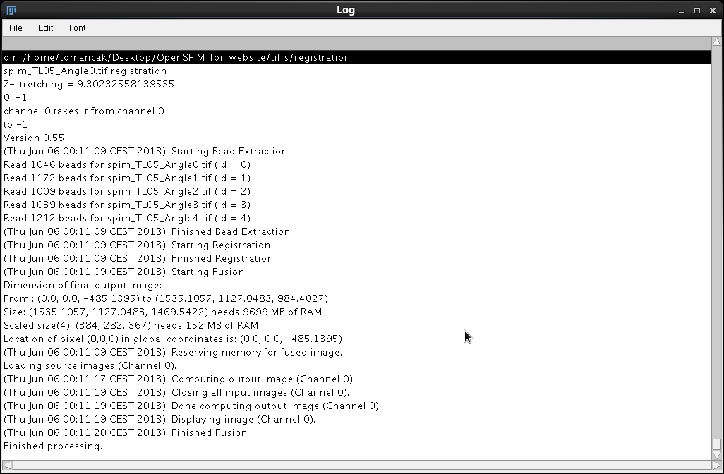
As before, let us annotate the output the fusion plugin sends to the Log window".
dir: /home/tomancak/Desktop/OpenSPIM_for_website/tiffs/registration spim_TL05_Angle0.tif.registration
Z-stretching = 9.30232558139535
The plugin identifies the registration files and reads in the z-scaling.
0: -1
channel 0 takes it from channel 0
tp -1
Version 0.55
(Thu Jun 06 00:11:09 CEST 2013): Starting Bead Extraction
Read 1046 beads for spim_TL05_Angle0.tif (id = 0)
Read 1172 beads for spim_TL05_Angle1.tif (id = 1)
Read 1009 beads for spim_TL05_Angle2.tif (id = 2)
Read 1039 beads for spim_TL05_Angle3.tif (id = 3)
Read 1212 beads for spim_TL05_Angle4.tif (id = 4)
(Thu Jun 06 00:11:09 CEST 2013): Finished Bead Extraction
(Thu Jun 06 00:11:09 CEST 2013): Starting Registration
(Thu Jun 06 00:11:09 CEST 2013): Finished Registration
It then repeats the registration steps. We will recall that the actual registration took very short time, once the beads are segmented reading them in and repeating the optimization is simpler then programming a specific function that would load the matrices from the files (apparently - Stephan?).
(Thu Jun 06 00:11:09 CEST 2013): Starting Fusion
Dimension of final output image:
From : (0.0, 0.0, -485.1395) to (1535.1057, 1127.0483, 984.4027)
Size: (1535.1057, 1127.0483, 1469.5422) needs 9699 MB of RAM
Scaled size(4): (384, 282, 367) needs 152 MB of RAM
Here we see the benefits of downsampling, the full resolution output image would need almost 10GB of RAM and thats only the final output excluding all intermediate steps - the actual memory footprint is several fold higher. One can easily run out of memory with this data. However scaled we are down to much more reasonable 152MB for the output image.
Location of pixel (0,0,0) in global coordinates is: (0.0, 0.0, -485.1395)
(Thu Jun 06 00:11:09 CEST 2013): Reserving memory for fused image.
Loading source images (Channel 0).
(Thu Jun 06 00:11:17 CEST 2013): Computing output image (Channel 0).
(Thu Jun 06 00:11:19 CEST 2013): Closing all input images (Channel 0).
(Thu Jun 06 00:11:19 CEST 2013): Done computing output image (Channel 0).
(Thu Jun 06 00:11:19 CEST 2013): Displaying image (Channel 0).
(Thu Jun 06 00:11:20 CEST 2013): Finished Fusion
Finished processing.
Now here is the action, the plugin loads the images, fuses them without doing any entropy evaluation, closes the input images and displays the output. Since we are working with 4 times down-sampled data it all takes only seconds.
A new window will pop-up. This is the Output that we will discuss in the next section.
Output and Evaluation
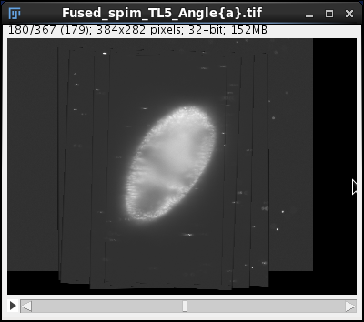
4 times downsampled fusion output, auto contrast adjusted
At end of the Run a new window pops up. Now we finally see our registered OpenSPIM data albeit heavily downsampled.
This is not exactly what we hoped for, there are lines and grey boxes everywhere and the resolution is poor. This is because we downsampled and turned off all fusion bells and whistles. When we scroll through the stack we nonetheless can see that the 5 views making up this time point have indeed been registered as there are no obvious discontinuities in the data and the entire embryo is covered.
We are looking at the data from the point of view of the reference view (in this case Angle0). This view hasn't been transformed, we are looking at the data as they were acquired, downsampled and degraded by averaging in the blurred data from other views (we did no content based weighting).
We will use this initial output to demonstrate the fundamental principle of the bead based multi-view registration. Let's turn this stack to look at it along the rotation axis. We do that by running Plugins->Transform->TransformJ->TransfromJ Turn and turning the fusion output stack around the x axis by 90 degrees.
When we now navigate through the turned stack we are looking approximately alongside the rotation axis. We see how the five individual view stacks overlap in the output volume and how the bounding box of that volume becomes consequently large.
We see also the elongated Point Spread Function (PSFs) of the beads. These axially elongated PSFs cross forming beautiful stars. Their presence around the specimen indicates that the registration was successful.
Cropping
In the next step of the fusion pipeline we will crop the output image as much as possible. Why? You may have noticed that the bounding box of the fused image is actually rather large (4 x 384x282x367). This is because we have rotated the input image stacks in 3d and the resulting cubic volume has to include them all. Saving output images in this form would increase the storage requirements by orders of magnitude. To reduce the storage footprint we will use this initial run of fusion to define a volume that fits the specimen most efficiently. It will also reduce memory requirements allowing us to run the fusion with full resolution images.
Note that in reality it makes sense to define the crop volume only after the time-lapse registration, because that will be the final output of the pipeline and the crop area has to be defined relative to that registration. However to preserve linearity we will describe cropping here.
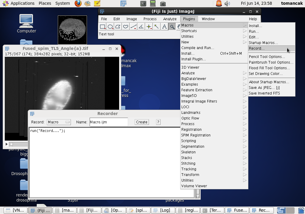
Screenshot of macro recorder, showing where to find it in Fiji menus and the recorder window which has just recorded the running of the macro recorder command (little recursion) |
Before you start cropping start a macro recorder. Macro recorder will open a window that will report the parameters of commands we run in Fiji. We will need it to note the coordinates of the bounding box. |
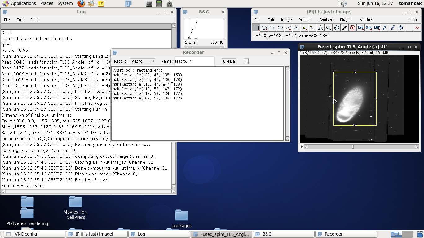 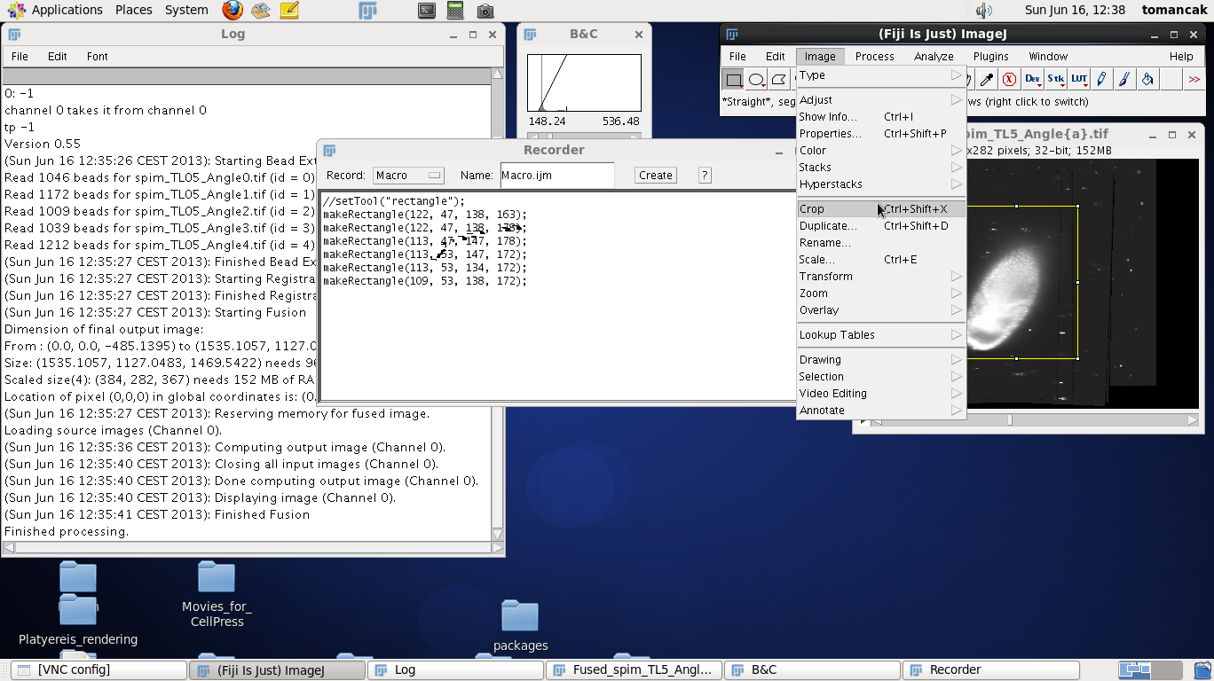 |
To define the crop area we click on the rectangle tool in the main Fiji window and make a rectangle around the contrast adjusted fused data. Move up and down through the z stack to make sure that the rectangle includes all the data. Modify the size of the rectangle by dragging the tiny boxes on the rectangle. Make the rectangle tight around the data but leave a few pixels buffer zone. Note that every time you adjust the rectangle a new command get recorded in the Recorder window, such as makeRectangle(109, 53, 138, 172);. The numbers have the following meaning:
Note that we will need those numbers - so either write them down or keep the Recorder window open, which is the point of running it in the first place. Now we run the Crop function from the Fiji menus which will crop the image to the size of the placed rectangle. |
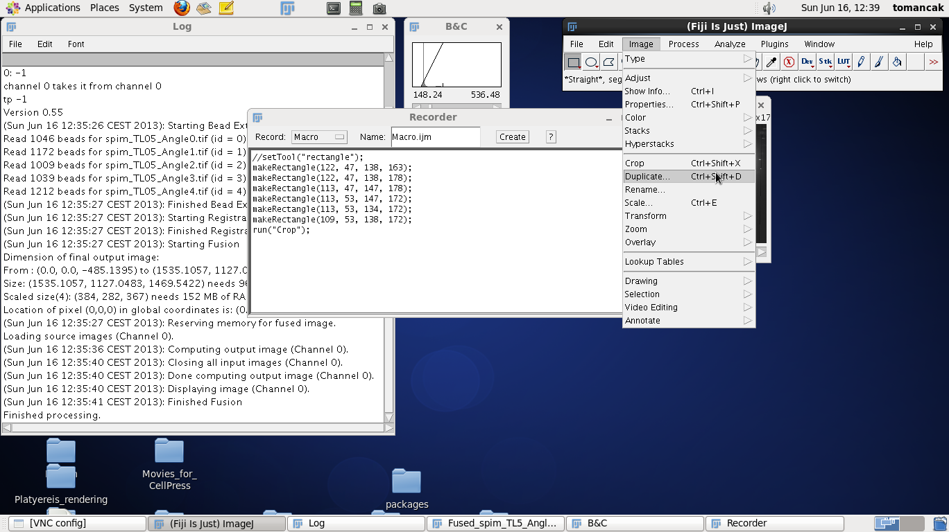 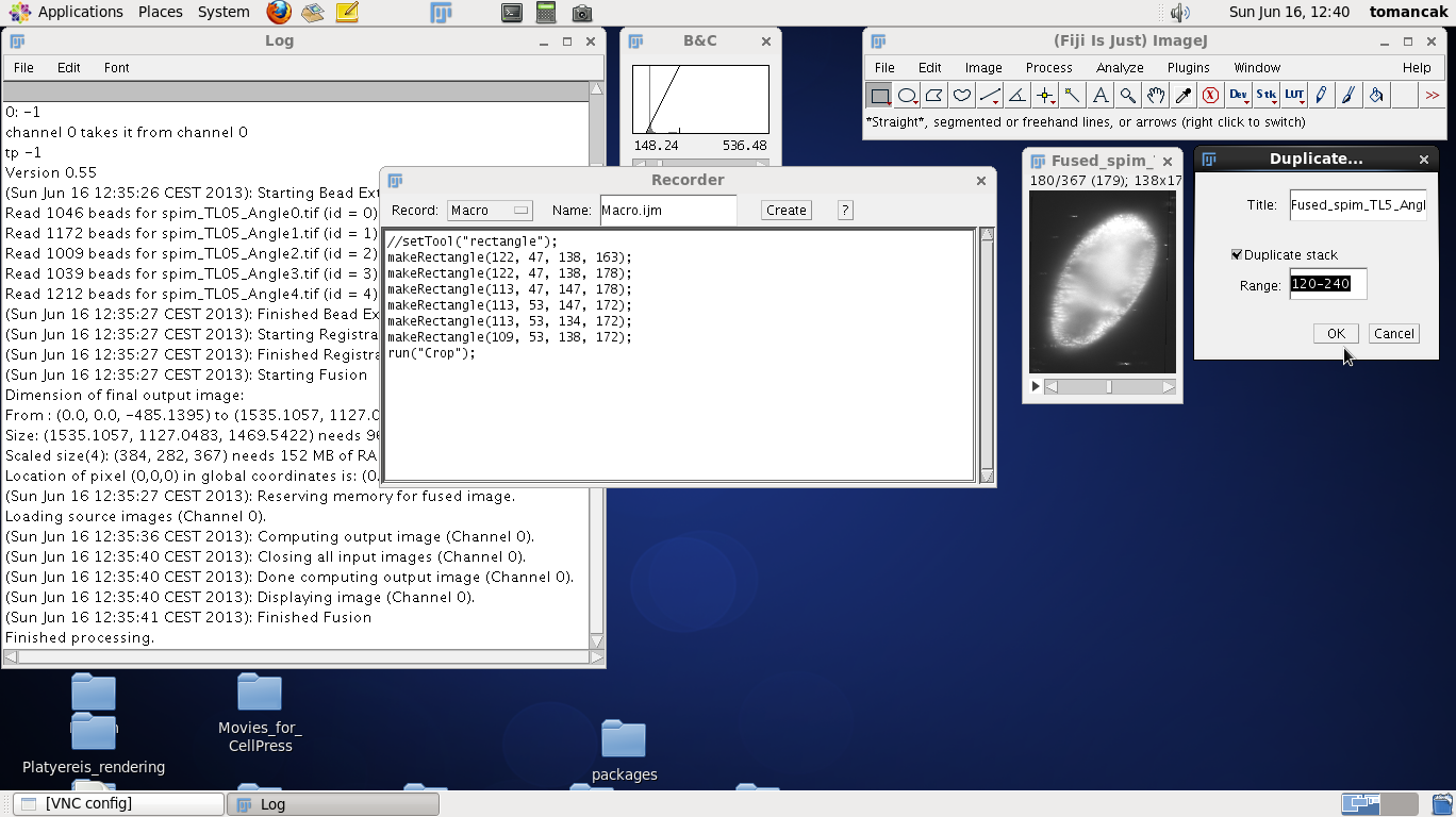 |
The cropped image is still too big in the z-direction. Once again move the z-slider up and down to determine at which z-index the data start and end. Remember the two z-indices (for this data roughly 120 and 240). Now to also record them we will run the command Duplicate stack from Fiji menus and fill in the numbers as shown on the screenshots to the right. Running the command will duplicate the stack and make it as small as possible without discarding any data. The range will also be recorded in the recorder as highlighted:
We are done with cropping, we can now proceed to run the fusion one more time with all the bells and whistles turned on taking advantage of the crop parameters to reduce the memory requirements. |
Final run
Now that we figured out the minimal crop area we will fuse the data at full resolution.
|
Launching content based multi-view fusion |
Start once again the Plugins->SPIM registration->Multi-view fusion plugin and click through the first two windows, the parameters should be pre-filled (unless you restarted Fiji in the meantime). | |
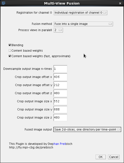
Screenshot of main fusion dialog with fusion parameters enabled and crop area filled, no downsampling |
Next we will specify some new parameters for fusion. We will use the individual registration because that is the only one we have (unless we have run time series registration before). We want to fuse into a single output image and we will this time process two views in parallel (On our super-duper computer we have enough memory to do them all at once, but it is not a realistic situation).
Click the Blending checkbox to turn on blending of intensities at the borders between views (otherwise there would be a visible line where one view abruptly ends). Select Content based weights (fast, approximate) over the full Content based weights, the difference is negligible and this will compute significantly faster. This time we will not downsample at all - 1 or 0 both signify this. Next we fill specify the cropping parameters. Alas these numbers on the screenshot do not look familiar. This is because we collected numbers in the previous cropping section on four times downsampled data. Therefore we have to multiply these number by a factor of four like this:
Finally we decide to save the data one directory per time-point and click OK to start processing. |
Lets annotate the output in the Log windows to understand what is going on
(Sun Jun 16 19:54:30 CEST 2013): Starting Bead Extraction
Read 1046 beads for spim_TL05_Angle0.tif (id = 0)
Read 1172 beads for spim_TL05_Angle1.tif (id = 1)
Read 1009 beads for spim_TL05_Angle2.tif (id = 2)
Read 1039 beads for spim_TL05_Angle3.tif (id = 3)
Read 1212 beads for spim_TL05_Angle4.tif (id = 4)
(Sun Jun 16 19:54:30 CEST 2013): Finished Bead Extraction
(Sun Jun 16 19:54:30 CEST 2013): Starting Registration
(Sun Jun 16 19:54:30 CEST 2013): Finished Registration
(Sun Jun 16 19:54:30 CEST 2013): Starting Fusion
Dimension of final output image:
From : (0.0, 0.0, -485.1395) to (1535.1057, 1127.0483, 984.4027)
Size: (1535.1057, 1127.0483, 1469.5422) needs 9699 MB of RAM
Cropped image size: 552x688x480
Needs 695 MB of RAM
We have reduced the memory requirements by cropping more then ten fold (from 9.6 GB to about 0.6 GB).
Location of pixel (0,0,0) in global coordinates is: (436.0, 212.0, -5.139496)
(Sun Jun 16 19:54:30 CEST 2013): Reserving memory for fused image.
(Sun Jun 16 19:54:30 CEST 2013): Unloading source images.
(Sun Jun 16 19:54:30 CEST 2013): Computing output image (Channel 0).
(Sun Jun 16 19:54:30 CEST 2013): Loading view: spim_TL05_Angle0.tif
(Sun Jun 16 19:54:32 CEST 2013): Loading view: spim_TL05_Angle1.tif
(Sun Jun 16 19:54:34 CEST 2013): Init isolated weighteners for views 0 to 1: (Average approximated Entropy using Integral images)
Computing Average approximated Entropy using Integral images for spim_TL05_Angle0.tif (id = 0)
Computing Average approximated Entropy using Integral images for spim_TL05_Angle1.tif (id = 1)
(Sun Jun 16 19:54:34 CEST 2013): Computing Integral Image
(Sun Jun 16 19:54:34 CEST 2013): Computing Integral Image
Initialize combined weighteners for for views 0 to 1 (Blending) (24 threads)
(Sun Jun 16 19:54:37 CEST 2013): Starting fusion for: spim_TL05_Angle0.tif
(Sun Jun 16 19:54:37 CEST 2013): Starting fusion for: spim_TL05_Angle1.tif
(Sun Jun 16 19:55:00 CEST 2013): Loading view: spim_TL05_Angle2.tif
(Sun Jun 16 19:55:02 CEST 2013): Loading view: spim_TL05_Angle3.tif
(Sun Jun 16 19:55:04 CEST 2013): Init isolated weighteners for views 2 to 3: (Average approximated Entropy using Integral images)
Computing Average approximated Entropy using Integral images for spim_TL05_Angle2.tif (id = 2)
Computing Average approximated Entropy using Integral images for spim_TL05_Angle3.tif (id = 3)
(Sun Jun 16 19:55:04 CEST 2013): Computing Integral Image
(Sun Jun 16 19:55:04 CEST 2013): Computing Integral Image
Initialize combined weighteners for for views 2 to 3 (Blending) (24 threads)
(Sun Jun 16 19:55:07 CEST 2013): Starting fusion for: spim_TL05_Angle2.tif
(Sun Jun 16 19:55:07 CEST 2013): Starting fusion for: spim_TL05_Angle3.tif
We decided to fuse two view at once and so we need altogether three rounds of sequential processing (0,1 followed by 2,3 and 5 below)
(Sun Jun 16 19:55:28 CEST 2013): Loading view: spim_TL05_Angle4.tif
(Sun Jun 16 19:55:30 CEST 2013): Init isolated weighteners for views 4 to 4: (Average approximated Entropy using Integral images)
Computing Average approximated Entropy using Integral images for spim_TL05_Angle4.tif (id = 4)
(Sun Jun 16 19:55:30 CEST 2013): Computing Integral Image
Initialize combined weighteners for for views 4 to 4 (Blending) (24 threads)
(Sun Jun 16 19:55:32 CEST 2013): Starting fusion for: spim_TL05_Angle4.tif
Computing final output image (Channel 0).
(Sun Jun 16 19:55:52 CEST 2013): Done computing output image (Channel 0).
(Sun Jun 16 19:55:56 CEST 2013): Finished Fusion
Finished processing.
The whole process took about 1.5 minutes. Now let's have a look at where to find the output.
The output goes by default to a subdirectory /output in the directory where we have the raw data.
cd output/
ls
5
The directory contains at the moment a single subdirectory named 5/ because we fused time point number 5 and said to save each time point to its own directory.
cd 5/
ls -1
img_tl5_ch0_z000.tif
img_tl5_ch0_z001.tif
img_tl5_ch0_z002.tif
img_tl5_ch0_z003.tif
img_tl5_ch0_z004.tif
img_tl5_ch0_z005.tif
img_tl5_ch0_z006.tif
img_tl5_ch0_z007.tif
img_tl5_ch0_z008.tif
img_tl5_ch0_z009.tif
.
.
That directory contains a series of tifs each representing one plane of the fused output volume. 480 files in total. These images can be opened in Fiji using File->Import->Image sequence or the entire directory can be simply dragged and dropped into onto Fiji's main window.
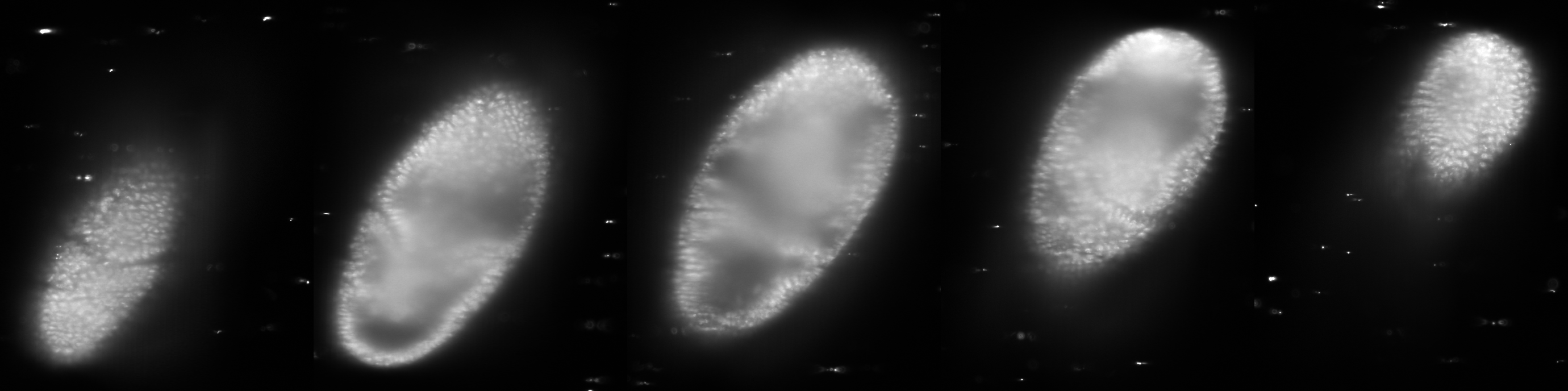
Slices through the fused full resolution output volume (step 80)
There are other ways to look at the data as we will see here. Note that the fused data are looking perhaps slightly worse compared to the raw data. This is primarily caused by two factors. First the content based fusion combined sharp and blurred information from different views by entropy based weighing and this is not perfect (see the next section deconvolution for a more advanced fusion approach). Second the embryo is alive and it moves, particularly at this stage of development (gastrulation) the movement is quite fast and it is not quite matched by the acquisition speed of OpenSPIM. I.e. by the time we acquire the fifth view that overlaps with the first views the cells may have moved. The only way to overcome that is to build a faster microscope or slow development down by lowering temperature.
Anyway, this is the final step of content based fusion of a single time-point. From here you can either continue to explore the deconvolution based fusion (right below) or you should switch to time series registration which is the next step of the SPIMage processing pipeline.
Deconvolution
The description of multi-view deconvolution plugin is available here. Deconvolution is still work in progress. Although it is already available in Fiji, it has not yet been published. I will make a detailed tutorial for it as soon as I find the time.