Sample raw data from Dresden's OpenSPIM
We will explain the entire SPIMage processing (SPIM image processing) pipeline using long-term time-lapse dataset acquired in Dresden during preparation of the OpenSPIM publication. We imaged Drosophila melanogaster embryos expression His-YFP in all cells from five angles every 6 minutes throughout embryogenesis - from gastrulation until the embryo started moving which is a sign of muscle contractions. The final processed and 3d rendered dataset looks like this:
Histone-YFP from gastrulation to beginning of muscle contraction from ventral, lateral and dorsal view
The entire multi-view time-lapse consists of 235 time points and the raw acquired ome.tiffs add up to 173 GB. Therefore, for the purposes of our tutorial we will be using the first 11 time-points of the time series.
DOWNLOAD the 2.3 GB zipped tar archive.
The tarball can be simply expanded into a working directory using
tar -xvzf OpenSPIM_Drosophila_10tp.ome.tiff.tar.gz
Each view consists of a stack of 51 images (imaged planes through the specimen 6 microns apart) saved as spim_TL<tt>_Angle<a>.ome.tiff where tt refers to zero padded time-points (01 - 235) and a refers to the five acquisition angles (0-4).
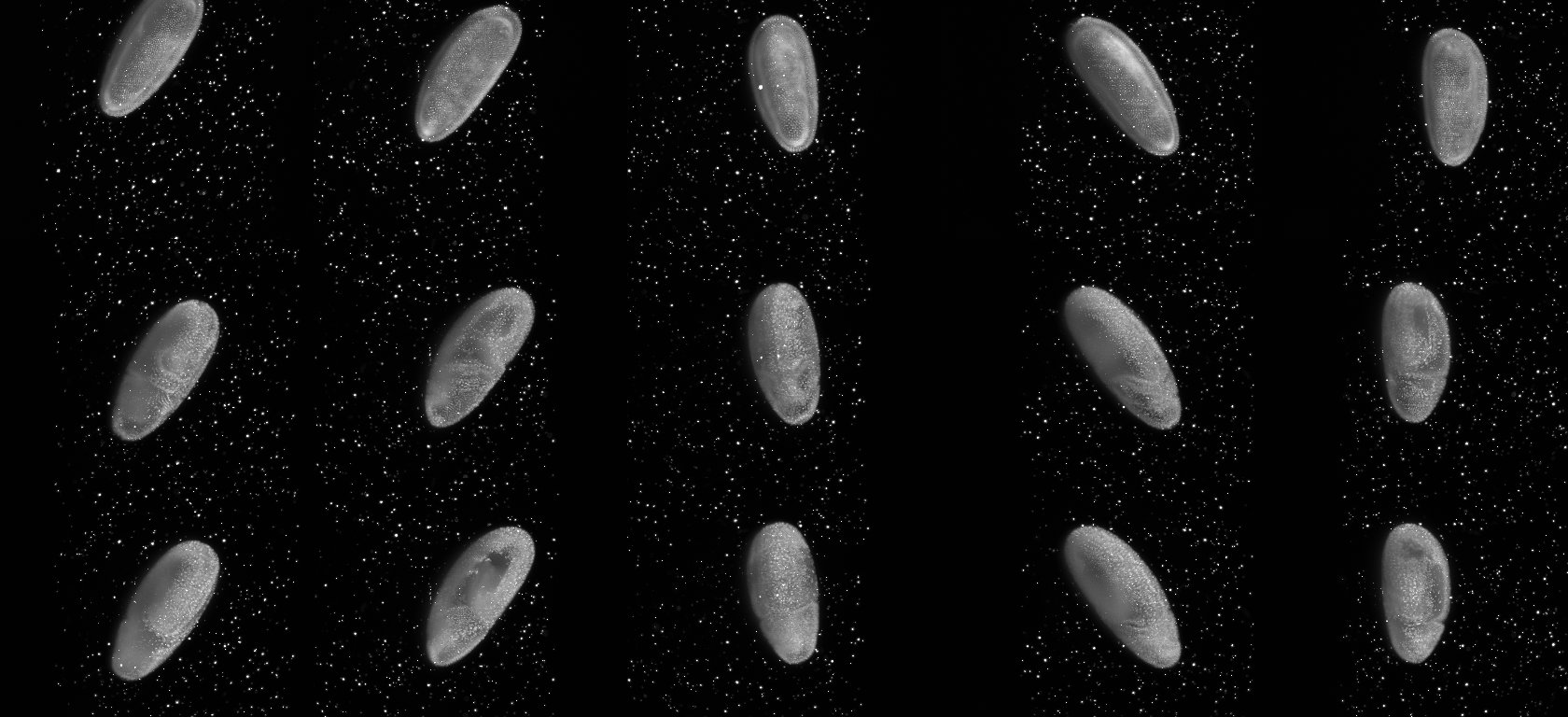
Max intensity projections 5 views (columns) from 3 time points
(0,5,10 rows) from sample OpenSPIM Dresden data
On the right we show maximum intensity projections for three time-points (rows) for each view (columns) separately. Note the beads surrounding the sample, the bead-free space outside the agarose column and the embryo specimen. In the first view of the first time point the embryo is partly outside the field of view. This is a feature not a bug. In OpenSPIM we set-up the angles quickly and approximately and adjust them after the acquisition of the first time-points. As one can see for time-points 5 and 10 the embryo is centered in the middle of the field of view.
Now that we have some sample data we can continue on in the SPIMage processing pipeline to the, hopefully temporary, pre-processing step.