Image Registration
Bead Based Registration
The first step in the SPIMage processing pipeline, after re-saving the ome.tiffs as .tif, is to register the views within each time point. We will use for that the bead based registration plug-in in Fiji. The principles of the plug-in are described on the Fiji wiki page SPIM registration method while the parameters are discussed in SPIM bead registration. Here we present a step by step recipe for performing the bead based registration on OpenSPIM data.
Input
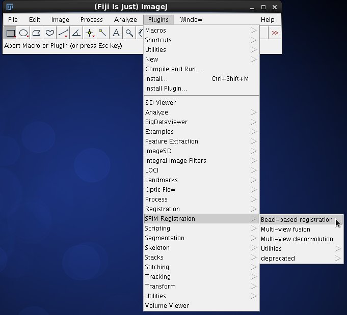
Screenshot of SPIM registration section of Fiji plugin menu First we start the plugin from Plugins->SPIM Registration->Bead based registration (or pressing letter l and typing SPIM etc.). Note that all SPIM related plugins are conveniently grouped in the plugins submenu SPIM Registration. Later on we will see how to use Multi-view fusion to combine registered views into a single output image and Multi-view Deconvolution for deconvolution mediated fusion which enhances image contrast and in some cases improves resolution. The plugins are linked to each other and share many parameters. I.e. if we first run registration and select the appropriate directories with data, these fields will be pre-filled for fusion unless, of course, we have restarted Fiji in the meantime. |
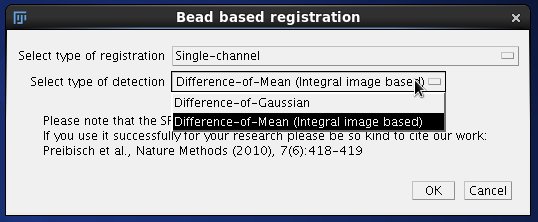
Screenshot of the first dialog of the bead based registration plugin In the following window we choose Single channel registration and select between two methods of localising the beads. Difference-of-Gaussian (DoG) is more precise however slower compared to Difference of Mean which takes advantage of integral images. In most cases Difference of Mean will be sufficient for registration of OpenSPIM data and so we will choose this option. Click OK to continue to the second dialog. |
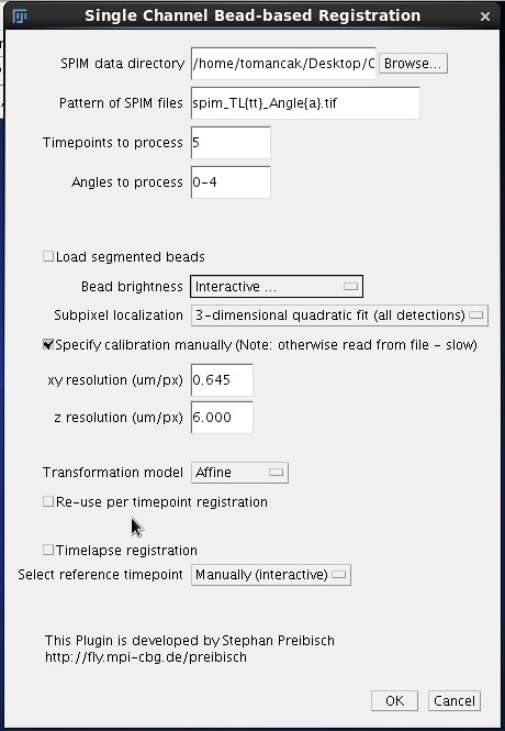
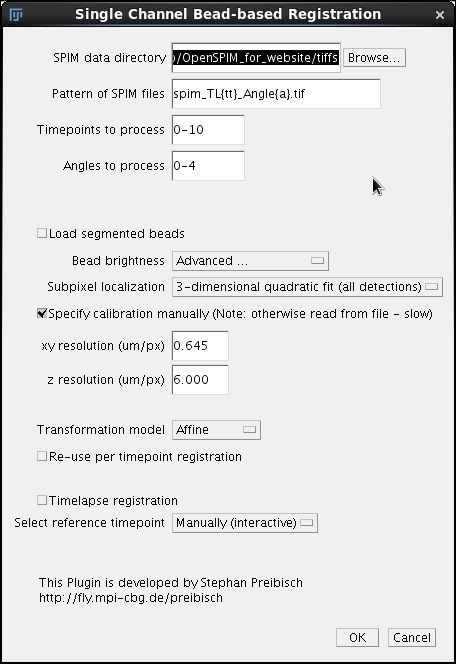
Screenshot of the second dialog of the bead based registration plugin Click Browse to locate the directory with the .tif files generated in the previous step of the pipeline. Enter the pattern of the files, where tt is a zero padded place holder for time points and a a zero padded placeholder for angles/views. If we have a three digit series (000 - 100) we use {ttt}; in case of our sample data that range from 0 to 10 we need tt as time point placeholder. Importantly, do not forget to adjust the extension to .tif. This is a common mistake at the default extension is for historical reason .lsm - a format used to store data from the Zeiss SPIM demonstrator. We will initially optimize the registration using time point 5. To register all time-points in the time series we would enter 0-10. The range does not need to start with 0 or 1. Discontinuous series is also possible, for example 1,5,10. Finally we specify the Angles to process, in our case 0-4 (0.1.2.3.4 = 5 angles). Any comma separated list will do, for instance 60,180, 235. In the second section of the dialog we need to initially pay attention only to the parameters affecting the initial segmentation of the bead. Bead Brightness is a pull down menu offering 6 options.
In our initial run we will select the option Interactive to play around with the threshold that is best suited for our data. The Subpixel localization is a pull down menu offering three option for more-or-less precisely localizing the beads
We will select 3-dimensional quadratic fit for our sample OpenSPIM data. For OpenSPIM data it is very important to select the Specify calibration manually checkbox and enter the xy and z resolution. For the sample OpenSPIM data discussed here the following parameters work.
Note that the important number here is the ration between the z and xy resolutions. In the case of OpenSPIM sample data it is 6/0.645 = 9.3023. We could also express the ratio as xy = 1 and z = 9.3023. The 9.0323 or z-scaling is an important number to remember and write down. It will also be stored as the value in the *.registration files as discussed below. We will need it during all subsequent steps. Finally we will examine the pull down menu Transformation model that offer three options
We will leave Affine as a useful and, in fact, necessary default for OpenSPIM data. That's it, we can for now safely ignore the remaining options of the dialog and proceed by clicking OK. |
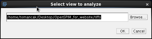
Dialog for selection of data file (view) for Interactive bead segmentation. Since we have selected the Bead brightness->Interactive the next dialog will ask us to select a time-point to perform the segmentation optimization on. Click Browse and locate the file spim_TL05_Angle0.tif and then press OK. |
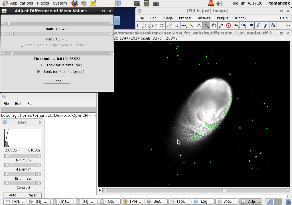
Desktop showing windows opened during interactive segmentation. After a short delay two windows will pop-up. In the browsable stack window the view selected in the previous step is shown and beads segmented using the current parameters are highlighted with small green circles. The parameters can be interactively changed in the Adjust Difference-of-Mean Values window. Typically we only need to play with the Threshold. The lower the threshold the more 'beads' are segmented. The goal here is to find a threshold where most beads are detected - ideally only once. We can examine the performance of a particular threshold by browsing through the stack and zooming in and out using the Fiji toolbar tools. We want to avoid the situation where several detections are shown for what appears to be a single bead and conversely when clearly visible beads are not detected at all. You will notice that the detections (the green circles) are not limited to beads but occur also around the nuclei inside the sample. As we will see later, these detection are spurious, not repeatable between views, and do not compromise the registration process. The search for the optimal threshold can be made easier by adjusting the contrast of the stack to see the beads better (window in the lower left corner, press CTRL-SHIFT-C and click on Auto). The threshold that works well for OpenSPIM sample data is 0.01 Once we identify a reasonable threshold we can click Done and start the registration process with the selected threshold. |
Run
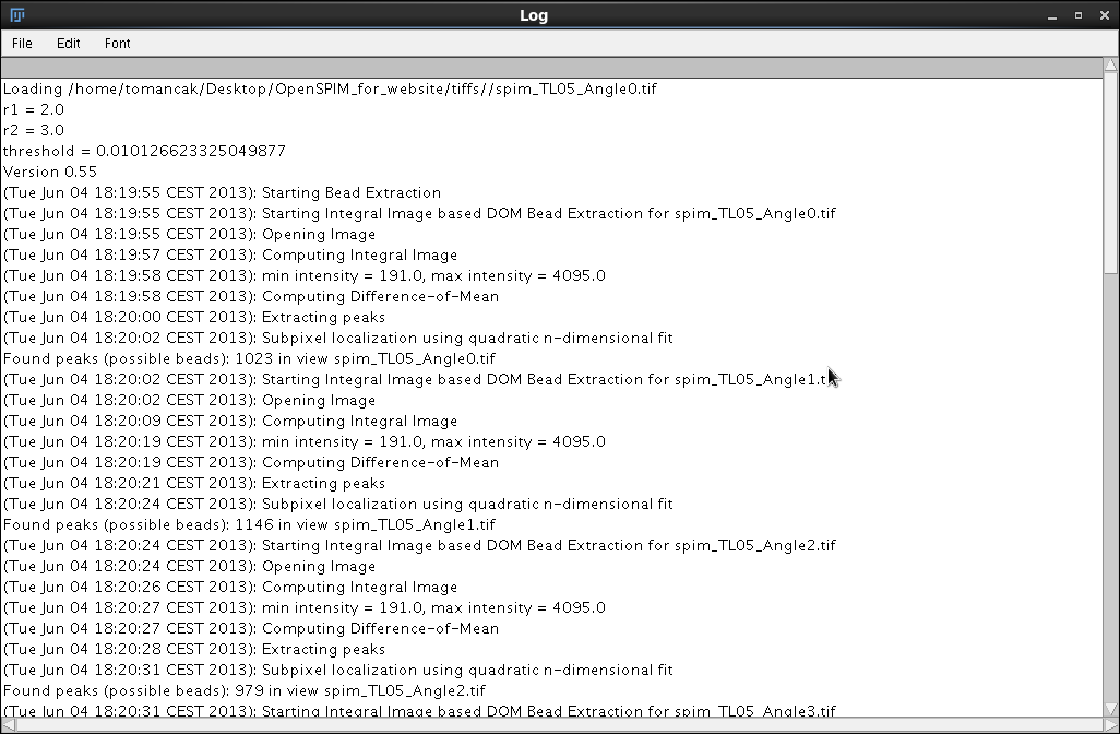
Screenshot of a Registration log window
The output of the registration plugin is not visual, it is limited to text messages in Fiji's Log window. However understanding the meaning of these messages is very important for optimization of the registration. The complete output of the registration of time-point 5 from OpenSPIM sample data is available here. Below we comment on the most important messages appearing in the output.
Loading /home/tomancak/Desktop/OpenSPIM_for_website/tiffs//spim_TL05_Angle0.tif
r1 = 2.0
r2 = 3.0
threshold = 0.010126623325049877
Here are the parameters (particularly the threshold) determined during the Interactive segmentation session described in the previous step.
Version 0.55
(Tue Jun 04 18:19:55 CEST 2013): Starting Bead Extraction
(Tue Jun 04 18:19:55 CEST 2013): Starting Integral Image based DOM Bead Extraction for spim_TL05_Angle0.tif
(Tue Jun 04 18:19:55 CEST 2013): Opening Image
(Tue Jun 04 18:19:57 CEST 2013): Computing Integral Image
(Tue Jun 04 18:19:58 CEST 2013): min intensity = 191.0, max intensity = 4095.0
(Tue Jun 04 18:19:58 CEST 2013): Computing Difference-of-Mean
(Tue Jun 04 18:20:00 CEST 2013): Extracting peaks
(Tue Jun 04 18:20:02 CEST 2013): Subpixel localization using quadratic n-dimensional fit
Found peaks (possible beads): 1023 in view spim_TL05_Angle0.tif
Processing of the first view spim_TL05_Angle0.tif started at 18:19:55 and ended 18:20:02, i.e. it took 7 seconds to find bead candidates for one view. The plugin reports 1023 possible beads. These include the detections inside the specimen. Only small percentage of these detections will be actually used in the registration (for details see SPIM registration method).
(Tue Jun 04 18:20:02 CEST 2013): Starting Integral Image based DOM Bead Extraction for spim_TL05_Angle1.tif
(Tue Jun 04 18:20:02 CEST 2013): Opening Image
(Tue Jun 04 18:20:09 CEST 2013): Computing Integral Image
(Tue Jun 04 18:20:19 CEST 2013): min intensity = 191.0, max intensity = 4095.0
(Tue Jun 04 18:20:19 CEST 2013): Computing Difference-of-Mean
(Tue Jun 04 18:20:21 CEST 2013): Extracting peaks
(Tue Jun 04 18:20:24 CEST 2013): Subpixel localization using quadratic n-dimensional fit
Found peaks (possible beads): 1146 in view spim_TL05_Angle1.tif
(Tue Jun 04 18:20:24 CEST 2013): Starting Integral Image based DOM Bead Extraction for spim_TL05_Angle2.tif
(Tue Jun 04 18:20:24 CEST 2013): Opening Image
(Tue Jun 04 18:20:26 CEST 2013): Computing Integral Image
(Tue Jun 04 18:20:27 CEST 2013): min intensity = 191.0, max intensity = 4095.0
(Tue Jun 04 18:20:27 CEST 2013): Computing Difference-of-Mean
(Tue Jun 04 18:20:28 CEST 2013): Extracting peaks
(Tue Jun 04 18:20:31 CEST 2013): Subpixel localization using quadratic n-dimensional fit
Found peaks (possible beads): 979 in view spim_TL05_Angle2.tif
(Tue Jun 04 18:20:31 CEST 2013): Starting Integral Image based DOM Bead Extraction for spim_TL05_Angle3.tif
(Tue Jun 04 18:20:31 CEST 2013): Opening Image
(Tue Jun 04 18:20:33 CEST 2013): Computing Integral Image
(Tue Jun 04 18:20:33 CEST 2013): min intensity = 191.0, max intensity = 4095.0
(Tue Jun 04 18:20:33 CEST 2013): Computing Difference-of-Mean
(Tue Jun 04 18:20:35 CEST 2013): Extracting peaks
(Tue Jun 04 18:20:37 CEST 2013): Subpixel localization using quadratic n-dimensional fit
Found peaks (possible beads): 1013 in view spim_TL05_Angle3.tif
(Tue Jun 04 18:20:37 CEST 2013): Starting Integral Image based DOM Bead Extraction for spim_TL05_Angle4.tif
(Tue Jun 04 18:20:37 CEST 2013): Opening Image
(Tue Jun 04 18:20:39 CEST 2013): Computing Integral Image
(Tue Jun 04 18:20:40 CEST 2013): min intensity = 191.0, max intensity = 4095.0
(Tue Jun 04 18:20:40 CEST 2013): Computing Difference-of-Mean
(Tue Jun 04 18:20:42 CEST 2013): Extracting peaks
(Tue Jun 04 18:20:45 CEST 2013): Subpixel localization using quadratic n-dimensional fit
Found peaks (possible beads): 1184 in view spim_TL05_Angle4.tif
Opening files took: 13 sec (27 %)
Computation took: 36 sec (73 %)
(Tue Jun 04 18:20:45 CEST 2013): Finished Bead Extraction
We found about 1000 bead candidates in each view. This number depends very much on the actual amount of beads used in the experiment, but as a rule of thumb, it should be in the thousands rather than hundreds. Only a small percentage of these detections will form descriptors repeatably detectable in different views and useful for registration. Hundreds of beads may not be enough. The segmentation of beads took 49 seconds on our souped up machine.
(Tue Jun 04 18:20:45 CEST 2013): Starting Registration
spim_TL05_Angle1.tif<->spim_TL05_Angle2.tif: Remaining inliers after RANSAC: 24 of 27 (89%) with average error 0.8298438414931297
This part of the log reports on the performance of the RANSAC (RANdom SAmple Consensus) algorithm. Between views Angle1 and Angle2 only 27 bead detection formed significant bead descriptor and 24 of these point to the same transformation model as determined by RANSAC. This is good.
spim_TL05_Angle3.tif<->spim_TL05_Angle4.tif: Remaining inliers after RANSAC: 15 of 17 (88%) with average error 0.7207672933737437
spim_TL05_Angle2.tif<->spim_TL05_Angle3.tif: Remaining inliers after RANSAC: 25 of 26 (96%) with average error 0.6098493030667305
spim_TL05_Angle0.tif<->spim_TL05_Angle1.tif: Remaining inliers after RANSAC: 20 of 21 (95%) with average error 0.8658423766493797
spim_TL05_Angle0.tif<->spim_TL05_Angle4.tif: Remaining inliers after RANSAC: 17 of 19 (89%) with average error 0.8551975593847387
spim_TL05_Angle1.tif<->spim_TL05_Angle4.tif: Remaining inliers after RANSAC: 23 of 23 (100%) with average error 0.7387010046969289
This is better, all bead descriptor point to the same transformation model.
spim_TL05_Angle0.tif<->spim_TL05_Angle2.tif: Remaining inliers after RANSAC: 25 of 26 (96%) with average error 1.035907996892929
spim_TL05_Angle2.tif<->spim_TL05_Angle4.tif: Remaining inliers after RANSAC: 52 of 53 (98%) with average error 0.6034472902806904
This is even better since here more beads are involved. The more bead descriptors survive RANSAC the better.
spim_TL05_Angle0.tif<->spim_TL05_Angle3.tif: Remaining inliers after RANSAC: 37 of 40 (93%) with average error 0.9902692207613502
spim_TL05_Angle1.tif<->spim_TL05_Angle3.tif: Remaining inliers after RANSAC: 44 of 47 (94%) with average error 0.5995832472531633
spim_TL05_Angle0.tif (id = 0) has 99 correspondences in 4 other views.
spim_TL05_Angle1.tif (id = 1) has 111 correspondences in 4 other views.
spim_TL05_Angle2.tif (id = 2) has 126 correspondences in 4 other views.
spim_TL05_Angle3.tif (id = 3) has 121 correspondences in 4 other views.
spim_TL05_Angle4.tif (id = 4) has 107 correspondences in 4 other views.
Overall we found true correspondences in all pairs of view. This is not absolutely necessary, however in general it is best to be able to link all views to each other for optimal registration results.
The total number of detections was: 5345
The total number of correspondence candidates was: 299
The total number of true correspondences is: 282
The number of true correspondences is the best indicator of registration success, the bigger the better. We can optimize the bead segmentation by trial and error, testing different thresholds, until the number of true correspondences does not change anymore.
Fixing tile spim_TL05_Angle0.tif (id = 0)
The Angle0 has been selected as a reference. It is the first Angle we specified in the Angles to process field in the second SPIM registration dialog. The reference view can be changed by changing the order of angles - for example 3,0-2,4 will set the reference view to Angle3. This angle will not undergo any transformation, all other angles will be transformed relative to it.
Successfully optimized configuration of 5 tiles after 258 iterations:
average displacement: 1.169px
minimal displacement: 1.052px
maximal displacement: 1.346px
Here the plugin reports results of global optimization. The average displacement is a good measure of the registration success. the lower the better. However it should be noted that it refers only to displacement of truly corresponding beads and thus the number is somewhat dependent on the number of true correspondences. The average for smaller number of beads will be lower but that does not necessarily mean that the registration is better. We will return to the issue of registration evaluation in the Fusion section of this tutorial.
Optimizer Matrices
spim_TL05_Angle0.tif (id = 0):
Transformation:
3d-affine: (1.0, 0.0, 0.0, 0.0, 0.0, 1.0, 0.0, 0.0, 0.0, 0.0, 1.0, 0.0)
Scaling: (1.0, 1.0, 1.0)
spim_TL05_Angle1.tif (id = 1):
Transformation:
3d-affine: (0.40029413, -0.017728202, -0.94824606, 647.0399, -0.025776416, 0.99945474, -0.028035998, 78.98084, 0.91382235, 0.015030926, 0.32484454, -485.3402)
Scaling: (1.0410335704042355, 0.9563661799258112, 1.0012564667399522)
The actual result of SPIM registration are these formidable looking 3x4 affine transformation matrices. This is linear algebra and there is no gentler way to break into it than the Khan Academy. As you can see, the first matrix is mostly zeros apart from the ones for scale along the x, y and z axis, this is the so-called identity matrix for the reference view that, as we mentioned before, will not be transformed. The second matrix for Angle1 describes the affine transformation that will transform the raw data of that view to the position in the world coordinate space of Angle0 that minimizes the displacement of corresponding bead descriptors. The Scalings are close to 1 indicating that our z-scaling factor 9.3023 was correct.
spim_TL05_Angle2.tif (id = 2):
Transformation:
3d-affine: (-0.7431537, -0.042439252, -0.6486701, 1351.3088, -0.04479293, 0.9994802, -0.011400312, 103.38013, 0.62969136, 0.0018952899, -0.80743754, -48.216476)
Scaling: (0.97164466699547, 1.039995886748908, 0.9993666835629822)
spim_TL05_Angle3.tif (id = 3):
Transformation:
3d-affine: (-0.86488324, -0.03760272, 0.5719731, 1263.6525, -0.0322361, 0.9994662, 0.0067903697, 75.966225, -0.5214333, -0.025284931, -0.83718777, 856.8579)
Scaling: (1.0407955347327127, 1.0029041568010506, 0.9802812833830724)
spim_TL05_Angle4.tif (id = 4):
Transformation:
3d-affine: (0.5062743, -0.0048624836, 0.857942, 126.564545, -0.0015900917, 1.0001556, -0.0052930415, 78.1325, -0.828062, -0.02390239, 0.56586677, 652.8654)
Scaling: (0.9650266222266568, 1.0369083125363359, 0.9963691154426817)
(Tue Jun 04 18:20:45 CEST 2013): Finished Registration
Finished processing.
The global optimization took only 5 seconds, showing that the most computationally expensive step of the registration pipeline is the segmentation of beads. If we were to use more precise and slower bead segmentation algorithm (DoG and Gauss-fit) the registration could take several minutes. With Difference-of-Mean and quadratic fit we were able to accomplish the registration in 50 seconds.
Output
The log output described in the previous section allows us to monitor the progress of the registration and if necessary optimize the parameters or diagnose problems. The true output of the registration that will be used in the Fusion step are three files per view created by the plugin in the registration directory.
registration/spim_TL05_Angle0.tif.beads.txt
registration/spim_TL05_Angle0.tif.dim
registration/spim_TL05_Angle0.tif.registration
registration/spim_TL05_Angle1.tif.beads.txt
registration/spim_TL05_Angle1.tif.dim
registration/spim_TL05_Angle1.tif.registration
registration/spim_TL05_Angle2.tif.beads.txt
registration/spim_TL05_Angle2.tif.dim
registration/spim_TL05_Angle2.tif.registration
registration/spim_TL05_Angle3.tif.beads.txt
registration/spim_TL05_Angle3.tif.dim
registration/spim_TL05_Angle3.tif.registration
registration/spim_TL05_Angle4.tif.beads.txt
registration/spim_TL05_Angle4.tif.dim
registration/spim_TL05_Angle4.tif.registration
The content of the files for Angle1 are available here
- spim_TL05_Angle1.tif.registration
- [spim_TL05_Angle1.tif.dim]((documents/Spim_TL05_Angle1.tif.pdf)
- [spim_TL05_Angle1.tif.beads.txt]((documents/Spim_TL05_Angle1.tif.beads.pdf)
The spim_TL05_Angle1.tif.registration contains information about the registration statistics such as number of detections, bead candidates, corresponding bead descriptors, the z-stretching used for the registration, etc. and the affine matrices in the following form
m00: 0.40029413
m01: -0.017728202
m02: -0.94824606
m03: 647.0399
m10: -0.025776416
m11: 0.99945474
m12: -0.028035998
m13: 78.98084
m20: 0.91382235
m21: 0.015030926
m22: 0.32484454
m23: -485.3402
m30: 0
m31: 0
m32: 0
m33: 1
model: AffineModel3D
...
z-scaling: 9.0323
The spim_TL05_Angle1.tif.dim contains information about the dimensions of the input image stacks
image width: 1344
image height: 1024
image depth: 51
and spim_TL05_Angle1.tif.beads.txt contains a long list of all detections and their properties (showing the first few lines below):
ID ViewID Lx Ly Lz Wx Wy Wz Weight DescCorr RansacCorr
0 1 408.13684 118.505554 3.1183574 408.13684 118.505554 3.1183574 0.0 0 0
1 1 95.8529 429.66003 3.4262538 95.8529 429.66003 3.4262538 0.0 0 0
2 1 71.95479 802.522 8.498448 71.95479 802.522 8.498448 0.0 0 0
3 1 408.45068 769.5576 9.81232 408.45068 769.5576 9.81232 0.0 188:4; 188:4;
4 1 960.3512 603.2773 10.9592 960.3512 603.2773 10.9592 0.0 0 0
5 1 840.4799 555.54315 14.765049 840.4799 555.54315 14.765049 0.0 0 0
6 1 816.0067 102.64633 16.194763 816.0067 102.64633 16.194763 0.0 377:3;647:0; 647:0;377:3;
The raw data together with the three files in the /registration directory form a unit which together represents the results of the registration pipeline.
spim_TL05_Angle0.tif
spim_TL05_Angle1.tif
spim_TL05_Angle2.tif
spim_TL05_Angle3.tif
spim_TL05_Angle4.tif
registration/spim_TL05_Angle0.tif.beads.txt
registration/spim_TL05_Angle0.tif.dim
registration/spim_TL05_Angle0.tif.registration
registration/spim_TL05_Angle1.tif.beads.txt
registration/spim_TL05_Angle1.tif.dim
registration/spim_TL05_Angle1.tif.registration
registration/spim_TL05_Angle2.tif.beads.txt
registration/spim_TL05_Angle2.tif.dim
registration/spim_TL05_Angle2.tif.registration
registration/spim_TL05_Angle3.tif.beads.txt
registration/spim_TL05_Angle3.tif.dim
registration/spim_TL05_Angle3.tif.registration
registration/spim_TL05_Angle4.tif.beads.txt
registration/spim_TL05_Angle4.tif.dim
registration/spim_TL05_Angle4.tif.registration
The fusion and deconvolution plugins take the raw data and apply the transformation from the registration files to continue the SPIMage processing. The entire unit can be moved to another location in the file system (the registration directory has to remain a subdirectory of where the raw data reside and keep its name).
Before we continue with the pipeline we need to make some decisions regarding the processing of the time lapse data.
Cross-road in SPIM plugins
At this point we have registered data for one time-point (5). We have not yet seen the data though since the output are the human unreadable transformation matrices. We can either decide to trust the log files and go ahead and use the same parameters for the registration of the rest of the time-points in our sample OpenSPIM timelapse and perform the timelapse registration or we continue playing with our one registered timepoint, fuse it, evaluate the results and then return to processing the rest of the timelapse. Both avenues are possible in the SPIMage processing pipeline. We recommend to first perform image fusion on one time point, evaluate the results and then return to the registration.
Nevertheless for the sample data we can just as well apply the parameters (threshold) to all timepoints in the series. As before we launch the Bead based registration plugin, leave the parameters in the first dialog unchanged and modify the second dialog as follows:
SPIM registration dialog for per time point registration of entire time-series In the field Timepoints to process we fill 0-10 which encompasses all timepoints in the sample timelapse. Under Bead brightness pull down we will select the Advanced option and click OK. |
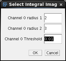
Direct entry segmentation parameters dialog A different intermediate dialog pops-up allowing us to directly enter the segmentation parameters. We enter 0.01 in the threshold field and click OK. A long stream of output in Log ensues while all 11 timepoints are consecutively processed. The registration of the time series took about 6 minutes and generated 3 x 11 = 33 files in the /registration directory. |
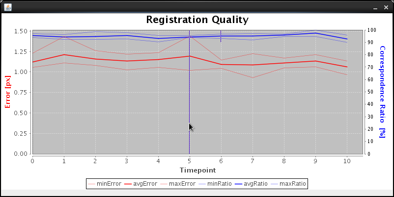
Plot of registration results for OpenSPIM sample data. The plugin plots the average, minimal and maximal displacement of corresponding bead descriptors as well as the RANSAC ratio of inliers (true/all correspondences) for all time-points. If you selected Manual (interactive) for the reference time-point, you will have to click using the mouse onto your time-point of choice that all others will be registered to. If you choose Automatic, the plugin will choose the time-point with the lowest error and highest number of inliers. Selecting Manually (specify) you will be queried for your choice of the reference time-point before the registration starts. This latter choice is especially useful for completely automatic processing, e.g. on a cluster. For such a small timelapse it is perfectly feasible to perform registration on a single computer consecutively. For longer timelapses we recommend using a cluster computer as described here. |