Note: This chapter describes some simple optical principles that should help you to align a SPIM. Most of these rules are approximations that are typically quite accurate for small angles. For a more thorough introduction it is recommended to read any established optics textbook.

Geometric Optics

We will start by briefly introducing some principles of geometric optics where light is thought of as an infinitely thin ray, or a bunch of rays. Each ray starts at a certain point (e.g. a light source) and progresses into space ad infinitum or until it hits a surface. At the surface (or interface between two media/materials) it may be:

• absorbed (i.e. vanishes)

• reflected, i.e. leaves the surface under an exit angle which equals the incident angle (see Mirrors below)

• refracted, i.e. is split into a reflected ray and a second ray penetrating the material, possibly changing directions. For the reflected ray, the exit angle θ_e again equals the incident angle θ_i, whereas for the refracted ray the exit angle θ_r is given by Snell's law and the refractive indices n₁ and n₂ of the two materials:

sin(θ_i)/sin(θ_r) = n₂/n₁

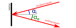
Mirrors

Mirrors are shiny surfaces that reflect a beam of light. The reflection is defined by the reflection law, which states the angle of the incident and the surface normal α_i equals the angle α_e of the exiting beam and the surface normal:

Mirror

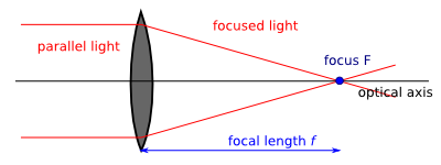
Lenses and parallel light

Lenses are curved glass surfaces that refract the light and focus a beam of parallel light onto a single spot called the focus F. The distance between the lens and the focus is called focal length f.

Lens

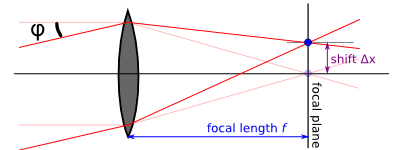
If the parallel light beam enters the lens under an angle φ, as in the image below, the focus F will be shifted perpendicularly to the optical axis by a distance Δx (Note: A shift on a flat plane is the ideal case -- which is nearly true for small shifts. For real lenses and larger shifts the shifted focus will move on a sphere centered in the center of the lens). The shift is given by a simple relation:

Δx = f·*tan*(φ)

Angled lens

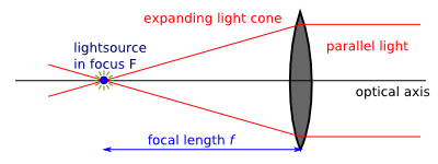
Another basic rule of optics states that:

Every beam path in an optical setup is reversible.

This means, e.g. for a lens, that it may either focus parallel light into a single spot, or alternatively collimate the light from a point source which is put into the focus. In the latter case the situation above is simply reversed (i.e. flip the image horizontally):

Reversed lens

Shifting the light source then also changes the angle φ under which the light leaves the lens.

In terms of Fourier optics, this finding makes a lens a Fourier transformer as it changes from a position (space) to an angle space, or vice versa.

Imaging with a lens

In the section above, we looked at what a lens does to parallel light or to point sources in the focal plane. These two cases are the most important ones when it comes to understanding the optics of OpenSPIM. But for the sake of completeness, we will also give the "standard sketch" of imaging with a lens:

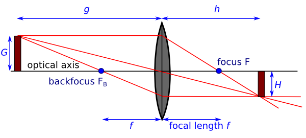
Lens imaging

Here an object of height G is positioned a distance g away from a lens (focal length f<g). Then a sharp image of height H is formed a distance h>f in front of the lens. For the size of the image and the distances holds the lens formula (an approximation for thin lenses!):

1/f = 1/G + 1/H

The image is magnified by a factor M:

M = h/g = H/G = f/(f-G)

Telescopes

Now we combine two lenses with focal lengths f and f' to form a telescope. A telescope is an optical assembly where the lenses are placed a distance f+f' apart. It can be used to expand or narrow the diameter of a beam of light.

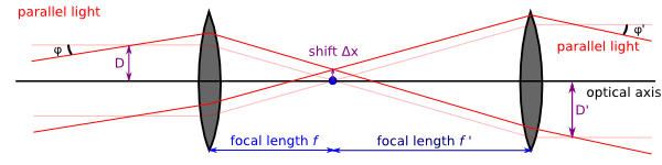
Telescope

As can be seen, the size of the incident parallel light beam is expanded by a factor M (magnification):

M = D' / D = f' / f

This can be understood using the principle of reversibility of optical beams (see above). The focus of the first lens can be seen as a point source for the second lens. The magnification is simply given by geometry.

To calculate the exit angle φ' for a given incident angle φ we can use the tangent law above:

Δx=f·*tan*(φ)=f'·*tan*(φ')

and therefore:

tan*(φ')/*tan*(φ) = f/f' = 1/M

Infinity Microscope

Now we take a second look at an assembly of two lenses, now forming an infinity microscope (which we use in the OpenSPIM to image the specimen onto the camera). Most of today's scientific grade fluorescence microscopes use this "infinity optics" principle:

1. The fluorescing sample is placed in the focal plane of the objective lens. Each point (fluorophore) in the sample can then be seen as a point source of light. The objective lens then converts the light from each of these points (at position x) into a parallel beam of light, exiting the objective under different angles φ(x).
2. A second lens (called tube lens) then converts these parallel beams back into an image in its focal plane, where the camera is placed. Alternatively an eyepiece can be used as a "magnifying glass" to observe this image by eye.

The whole setup looks like this:

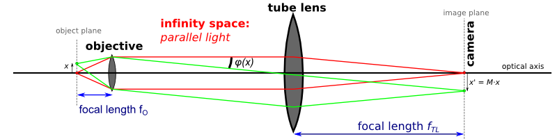
Infinity microscope

The magnification M=x'/x can again be easily calculated using the tangent law for lenses stated above. From:

x = f_O·*tan*(φ(x))* and *x'= f_TL·*tan*(φ(x))

follows that:

M = x'/x = f_TL/f_O

Note that we never used the distance between the objective and tube lens. In fact this distance does not play a major role for the imaging in an infinity microscope (If it is too long, the parallel beams expand too much and you will loose intensity in the image).

The space between the objective and tube lens is called "infinity space", because the image is focused "in infinity" here (i.e. we have parallel beams of light). The advantage of this is that we can easily introduce any planar optical elements (fluorescence filter, dichroic mirrors ...) without disturbing the optical properties of the microscope.

Gaussian Beam Optics

Definition of Gaussian Beams

So far we covered basic geometric optics, i.e. light was thought of as (infinitely thin) rays in space (or a whole bunch of these). Now we look at a more realistic model, where light is described as beams with a lateral intensity distribution. We will only cover basic principles of Gaussian beams, as they are the most common optical beams and have direct application to SPIM. The light exiting a laser is typically a Gaussian beam (then also called TEM00 mode) and the light sheet can be approximated as one. More details can be found e.g. in the Wikipedia articles below or the references at the end of this page:

• Gaussian Beam
• Gaussian Optics

The following shows the intensity distribution of a Gaussian beam behind a lens. The yellow lines show the rays of geometric optics.

Gaussian beam

As you can see, the intensity has a maximum with a certain width in the focus. Laterally the beam shows a 2D Gaussian profile. The intensity distribution in the whole beam can be described as a Gaussian function with position-dependent width w(z):

Beam intensity

Here z is the position along the direction of propagation and r is the lateral position. A typical laser beam is rotationally symmetric, thus r is the distance from the beam center (r²=x²+y²). When the light sheet should be described, the Gaussian beam is no longer rotationally symmetric but we can set r=y or r=x, respectively. The z-position dependent beam width w(z) is defined as::

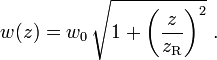
Beam width

with the Rayleigh length or depth of focus (λ is the wavelength of the light) defined as:

Rayleigh length/Depth of focus

This variable describes the range after which the center intensity I(0,z) has dropped to half its maximum value on the one hand and on the other hand the z-range through which the light cone does not expand strongly (w(z_R)=1.44·w₀). The intensity I(r,z) is plotted in the image above, the meaning of the quantities is shown in the next image:

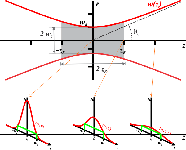
Focus

The description of a laser focus with Gaussian optics is valid for low NA lenses (typically NA<<1). For high NA lenses (as e.g. the projection and detection objective in an OpenSPIM) it is still a good approximation, although the focus will actually look more complex (e.g. with side lobes). Especially the relation for the depth of focus:

Rayleigh length/Depth of focus

still describes the light sheet of the OpenSPIM. The most important consequence of this equation for us is, that the width of the light sheet w₀ and the depth of focus z_R are interrelated:

The thinner the light sheet is, the shorter its depth of focus, i.e. the area in which its width does not change strongly, and which can therefore be used for imaging.

Beam Divergence and Numerical Aperture

Another parameter important for a Gaussian beam is its opening angle θ₀ which is approximately given in radians by:

θ₀ = λ / (π·w₀)

If the Gaussian beam is focused by a lens of a given numerical aperture NA we then have:

NA = n·sin(θ₀)

where n is the refractive index of the medium in which the beam is focused (e.g. n=1 for air or n=1.33 for water). Combining these two equations we can also estimate the minimal size of focus that can be achieved with a given lens (of given NA). We use the paraxial approximation which basically states that the angles θ₀ are small (compared to 1) and therefore θ₀=sin(θ₀). Then we get:

NA/n = λ / (π·w₀)

which yields:

w₀ = n·λ / (π·NA) = 0.32·n·λ / (π·NA)

So e.g. for a NA=0.03 projection lens, we get a focus size at λ=488nm in water (n=1.33) of w_0,NA0.03 = 1.33·0.488µm / (π·0.03) = 6.9µm. The according Rayleigh length is z_R=306µm

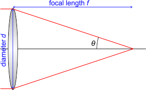
The numerical aperture of a lens is also determined by its diameter d and focal length f:

NA = d / (2·f)

Note however that the diameter d is not necessarily the true diameter of the lens. If the light beam before the lens is smaller than the lens' diameter, the effective NA of the lens is reduced accordingly. So if e.g. only half the diameter of an NA0.03 lens is illuminated (full illumination, see above), its effective NA is reduced by a factor of 2 to NA=0.015. Then we get the following focus width and Rayleigh length:

w_0,NA0.015 = 1.33·0.488µm / (π·0.015) = 13.8µm and z_R=1221µm

Note: The beam widths w₀ derived in the last paragraph give the length over which the intensity drops to 1/e²=13.5% of the center intensity. Often the full width at half maximum (FWHM) is used as a measure of beam width. These two are equivalent and can be converted from one to the other using this equation:

FWHM = w₀·ln(2) = w₀·0.693

The following approximations are very useful but only rigorously valid for small opening angles θ<<1 or NA<<1. In the OpenSPIM they can directly be used for the relais telescope lenses of f=25mm and f=50mm used to increase/decrease the size of the laser beam (diameter typically w₀=1mm, so NA=0.01-0.02). For the projection lens, creating the light sheet, or the detection objective, diffraction effects have to be taken into account. Here estimates like

FWHM=0.51·λ/NA* or accordingly *w₀=0.74·λ/NA

for the resolution of a fluorescence microscopy (point source) can be used (see e.g. Wikipedia: Optical resolution or Microscope Resolution in the german Wikipedia for further details).

Literature

You might want to read the following textbooks and journal articles for further information:

• Textbooks:
  • Bahaa E. Saleh and Malvin Carl Teich. Fundamentals of photonics., New York: Wiley, 1991.
• Journal articles:
  • K. Greger, J. Swoger, E. H. Stelzer: "Basic building units and properties of a fluorescence single plane illumination microscope". In: Review of scientific instruments. 78(2), 2007, p. 023705, PMID 17578115.